For my work with BIMI, I am working on developing an index of service accessibility. As part of this, I need to generate a lot of travel-time buffers around points: basically, if you start at a location and drive the speed limit in any direction, what is the polygon that you can access? These are called isochrones, and I’m using the Open Source Routing Machine and OpenStreetMap data to generate them.
Eventually, when the research is a little further along, I’ll do a post on how this process works—I learned a lot setting up OSRM and OSM and it’s worth putting it out on the internet for any OSRM newbies.
This post is specifically about how I sped up the OSRM function
osrmIsochrone. The package function is optimized for large-area
accuracy (I think), but since our buffers are relatively small (30
minutes driving) we can let go of one specific thing. No shade on the
OSRM developers, but I was able to speed this up quite a lot.
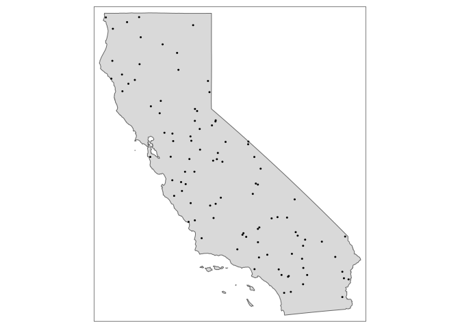
Our setup: We are putting a 30-minute driving buffer around 100 points randomly dropped in California:
library(sf)
library(tmap)
set.seed(4949)
CA_shp <- tigris::states(cb = TRUE, class = "sf") %>%
  filter(NAME == "California")
CA_pts <- st_set_geometry(data.frame(id = 1:100), st_sample(CA_shp, 100))
tm_shape(CA_shp) +
  tm_polygons() +
  tm_shape(CA_pts) +
  tm_dots()
Let’s set up OSRM:
library(osrm)
options(osrm.server = "http://0.0.0.0:5000/", osrm.profile = "driving")
I find it easiest for parallelization (which I’ll get to later) to write the process of generating isochrones in a function:
fx_base <- function(i, pts) {
  message(paste("Running location", i))
  tryCatch({
    return(st_set_geometry(pts[i,],
                           osrm::osrmIsochrone(
                             loc = pts[i,],
                             breaks = c(30),
                             res = 60,
                             returnclass =  "sf") %>%
                             filter(max == 30) %>%
                             st_geometry()))
  }, error = function(e) {
    message(paste("Failure at location", i, ":", e))
    print(pts[i, ])
    return()
  })
}
What this function does is take an index (as you’ll see, we’ll loop
through 1:nrow(CA_pts)) and the CA_pts object, get the isochrone
around that point, and return the original entry with the new geometry.
The osrmIsochrone function doesn’t preserve any of the attributes
passed, so this method returns the attributes of the original point with
the new buffer. We will eventually rbind them all together.
library(tictoc)
tic()
suppressMessages({
  CA_isochrones_base <- map(1:nrow(CA_pts), ~fx_base(., CA_pts))
  CA_isochrones_base <- data.table::rbindlist(CA_isochrones_base) %>% st_as_sf
  })

isochrones_base_time <- toc()
## 305.853 sec elapsed
This took about 5 minutes to run 100 points. This is fine for a small operation, but really a pain for a bigger one! Some values will fail. That’s okay– debugging that is a pain and ususally just means that there’s no road that gets to that point. And I know it’s weird that I’m using tidyverse syntax on SF with a data.table command– it works, don’t fight it!
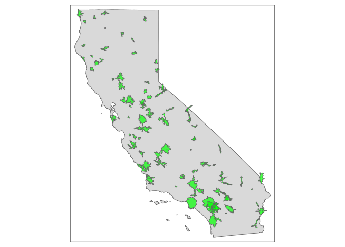
Here’s what they look like:
tm_shape(CA_shp) +
  tm_polygons() +
  tm_shape(CA_isochrones_base) +
  tm_polygons(col = "green", alpha= 0.7)
I can’t figure out how to put code profiling in an r markdown document
(at least) one that is static, but the output of profvis makes it look
like st_make_grid is eating up a lot of computation time. Some things
take longer, like i/o and fromJSON, but I can’t really do anything
about those.
My understanding of the algorithm is that it takes the input point, creates a grid of points on top, and evaluates the time from the input point to each point; it then draws a contour around all points that are below a certain travel time. However, the way it does that grid of points is markedly ineffecient. From the source code (many things are cut out):
function (loc, breaks = seq(from = 0, to = 60, length.out = 7),
    exclude = NULL, res = 30, returnclass = "sp") {

  ...
  ...

    if (options("osrm.profile") == "walk") {
        speed = 10 * 1000/60
    }
    if (options("osrm.profile") == "bike") {
        speed = 20 * 1000/60
    }
    if (options("osrm.profile") == "driving") {
        speed = 130 * 1000/60
    }
    dmax <- tmax * speed
    sgrid <- rgrid(loc = loc, dmax = dmax, res = res)
    lsgr <- nrow(sgrid)
    f500 <- lsgr%/%300
    r500 <- lsgr%%300
    listDur <- list()
    listDest <- list()
    if (getOption("osrm.server") != "http://router.project-osrm.org/") {
        sleeptime <- 0
    }
    else {
        sleeptime <- 1
    }
    if (f500 > 0) {
        for (i in 1:f500) {
            st <- (i - 1) * 300 + 1
            en <- i * 300
            dmat <- osrmTable(src = loc, dst = sgrid[st:en, ],
                exclude = exclude)
            durations <- dmat$durations
            listDur[[i]] <- dmat$durations
            listDest[[i]] <- dmat$destinations
            Sys.sleep(sleeptime)
        }
        if (r500 > 0) {
            dmat <- osrmTable(src = loc, dst = sgrid[(en + 1):(en +
                r500), ], exclude = exclude)
            listDur[[i + 1]] <- dmat$durations
            listDest[[i + 1]] <- dmat$destinations
        }
    }
    else {
        dmat <- osrmTable(src = loc, dst = sgrid, exclude = exclude)
        listDur[[1]] <- dmat$durations
        listDest[[1]] <- dmat$destinations
    }
    ...
    ...

}
The long and short of what I did is cut out this loop that contains for
(i in 1:f500) ...:
er_osrmIsochrone <- function(loc, breaks = c(30), exclude = NULL, res = 30, returnclass = "sf"){
  ...
  ...

   rgrid <- function(loc, dmax, res){
    # create a regular grid centerd on loc
    boxCoordX <- seq(from = sf::st_coordinates(loc)[1,1] - dmax,
                     to = sf::st_coordinates(loc)[1,1] + dmax,
                     length.out = res)
    boxCoordY <- seq(from = sf::st_coordinates(loc)[1,2] - dmax,
                     to = sf::st_coordinates(loc)[1,2] + dmax,
                     length.out = res)
    sgrid <- expand.grid(boxCoordX, boxCoordY)
    sgrid <- data.frame(ID = seq(1, nrow(sgrid), 1),
                        COORDX = sgrid[, 1],
                        COORDY = sgrid[, 2])
    sgrid <- sf::st_as_sf(sgrid,  coords = c("COORDX", "COORDY"),
                          crs = st_crs(loc), remove = FALSE)
    return(sgrid)
  }

  oprj <- st_crs(loc)
  loc <- loc[1,]
  loc <- st_transform(loc, 3857)
  row.names(loc) <- "0"

  # max distance mngmnt to see how far to extend the grid to get measures
  breaks <- unique(sort(breaks))
  tmax <- max(breaks)
  if(options('osrm.profile')=="walk"){
    speed =  10 * 1000/60
  }
  if(options('osrm.profile')=="bike"){
    speed =  20 * 1000/60
  }
  if(options('osrm.profile')=="driving"){
    speed =  130 * 1000/60
  }
  dmax <- tmax * speed
  sgrid <- rgrid(loc = loc, dmax = dmax, res = res)

  # dmat <- osrmTable(src = loc, dst = sgrid, exclude = exclude)
  dmat <- osrmTable(src = loc, dst = sgrid)
  durations <- dmat$durations
  destinations <- dmat$destinations
  ...
  ...
}
There are a few other operations, and you can view the full source code here.
Let’s test how fast it is:
source("er_osrmIsochrone.R")
fx_er <- function(i, pts) {
  message(paste("Running location", i))
  tryCatch({
    return(st_set_geometry(pts[i,],
                           er_osrmIsochrone(
                             loc = pts[i,],
                             breaks = c(30),
                             res = 60,
                             returnclass =  "sf") %>%
                             filter(max == 30) %>%
                             st_geometry()))
  }, error = function(e) {
    message(paste("Failure at location", i, ":", e))
    print(pts[i, ])
    return()
  })
}

tic()
suppressMessages({
  CA_isochrones_base <- map(1:nrow(CA_pts), ~fx_er(., CA_pts))
  CA_isochrones_base <- data.table::rbindlist(CA_isochrones_base) %>% st_as_sf
  })

isochrones_er_time <- toc()
## 229.679 sec elapsed
That’s not a bad speed up! Almost a minute and a half less. However, the real advantage comes when you have thousands of points and want to run them in parallel:
library(parallel)
CA_pts <- st_set_geometry(data.frame(id = 1:10000), st_sample(CA_shp, 10000))
tic()
  out <- suppressMessages({mclapply(1:10000, function(i) {fx_base(i, CA_pts)}, mc.cores = 16)})
isochrones_base_parallel_time <- toc()
## 2344.035 sec elapsed
tic()
  out <- suppressMessages({mclapply(1:10000, function(i) {fx_er(i, CA_pts)}, mc.cores = 16)})
isochrones_er_parallel_time <- toc()
## 1664.152 sec elapsed
In this toy case it’s not a huge speed up (about 30%), but on our applied problem, I was able to cut a 2-hour method down to 30 minutes. And that’s not nothing!
Final note: I believe that if you lower the resolution, this difference matters less. So this is all scale dependent.