My first post was a
lot of fun but I wanted to do a real post on something academic.
I’m working my way through old markdown scratch notebooks to fill out
this blog, and I’ll admit that this one is much less charming! Something
I’ve struggled with is simulating good spatial data for testing; it’s
really hard to come up with true autocorrelated data. The easiest way
I’ve found is with NIMBLE.
Let’s work with the CA counties dataset:
invisible({capture.output({CA_shp <- tigris::counties(state = "CA", cb = TRUE, class = "sf", refresh=TRUE)})})
suppressMessages(qtm(CA_shp))
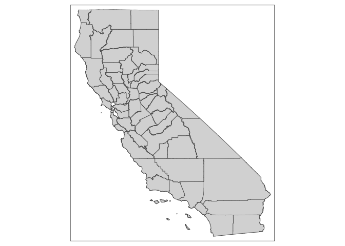 I
love the tmap package for plotting. It’s ggplot-style graphics are super
easy (with a few quirks– no variable alpha??) and the interactive
leaflet plotting is a breeze. The
tigris and related
tidycensus packages are
far and away the easiest ways to get US shapefiles and census/ACS data.
Seriously great!
I
love the tmap package for plotting. It’s ggplot-style graphics are super
easy (with a few quirks– no variable alpha??) and the interactive
leaflet plotting is a breeze. The
tigris and related
tidycensus packages are
far and away the easiest ways to get US shapefiles and census/ACS data.
Seriously great!
On the NIMBLE website there is a great example of how to simulate data. Such a cool package! Although I’ve mostly used it for its R-native implementation of Bugs, this is super helpful.
Let’s first talk about autoregressive distributions. The simplest one is the intrinsically autoregressive (IAR) distribution:
I think this is the simplest spatial distribution but it is far from perfect. Each observation is assumed to be normally distributed with mean equal to the average of its neighbors and with some constant variance. The main benefit here is that there is no weird “””““autocorrellation””””” parameter (like in other models, see below and Banerjee, Carlin, and Gelfand 2015 for a really great description of why this parameter isn’t really autocorrelation), but it doesn’t integrate; hence it can only be used as a prior. That’s why we love bayesian models for spatial data, right? Think about it: if you define each observation as a function of its neighbors, then there’s no ‘reference’ point setting the overall threshold, only the relative values. It also assumes stationarity and doesn’t let variance vary spatially, but I’m sure that could be built in as well. I’ve never been able to demonstrate this conclusively, but I think that the IAR model is best when there is a super strong spatial pattern.
Another benefit: I think the conditional specification above is easily the most interpretable of the spatial distributions. I don’t think there’s any ambiguity what’s going on there.
However, as mentioned above, this doesn’t integrate. It works great as a prior, but you can’t simulate from it. For that, we turn to the proper conditionally autoregressive distribution (CAR):
The funky thing here is the addition of γ, the autocorrelation paramter. This isn’t really autocorrelation in the traditional sense: as you can see, it’s really a “weight” for averaging the global mean μi and the autoregressive part. C is a weight matrix. I don’t love this distribution but we need it to simulate stuff.
To use the CAR distribution in NIMBLE/BUGS, we need to get the shapefile into a not-so-user-friendly format.
I was about to write up this kind of ugly code that does it, but it looks like there is a function that will do it for you! Thanks NIMBLE team.
Here’s code for that:
# help('CAR-Normal')
adj <- st_touches(CA_shp)
adj <- as.carAdjacency(adj)
num <- adj$num
adj <- adj$adj

set.seed(4949)

simCode <- nimbleCode({
  phi[1:n_counties] ~ dcar_proper(mu = mu[1:n_counties],
                                   adj = adj[1:n_adj], num = num[1:n_counties],
                                   tau = tau, gamma = gamma)

})

n_counties <- nrow(CA_shp)
inits <- list(phi = rep(0, n_counties))
simModel <- nimbleModel(code = simCode,
                        constants = list(n_counties = n_counties,
                                         adj = adj,
                                         n_adj = length(adj),
                                         num = num,
                                         tau = 0.0001,
                                         gamma = 0.99,
                                         mu = rep(0, n_counties)),
                        inits = inits)

nodesToSim <- simModel$getDependencies(c("phi"),self = T, downstream = T)
nodesToSim

## [1] "phi[1:58]"

simModel$simulate(nodesToSim)
simModel$phi

##  [1]  -53.758350   16.272210   49.363659  -94.573606   41.575196   18.959481
##  [7]  -36.990274  -32.260803   26.527266  -12.892487   30.424555 -105.271416
## [13]   71.155071  -56.552675 -148.938929 -143.035131    3.736508  -34.842856
## [19]   32.391517   65.546338  -35.344577  -59.731634  -47.512434  -46.274179
## [25]    4.975623   10.512559  -60.089720  -35.561165  -81.369520  -44.109275
## [31]  -11.438141   30.384663  -20.920760  -76.739383  -45.829361  -18.625771
## [37]   62.968067 -115.825910  -43.604169  -70.065963   17.311281   -2.570290
## [43]  -70.876395  -10.286491  -91.077975  -25.858164   11.890870  -52.833355
## [49]  -31.662219  -85.982585  -32.819344    9.782654   68.243890   74.069167
## [55] -119.381262   61.195767  -90.106324   -9.505612

CA_shp$phi <- simModel$phi
CA_shp %>% tm_shape() + tm_polygons(col =c("phi"), style = "cont")
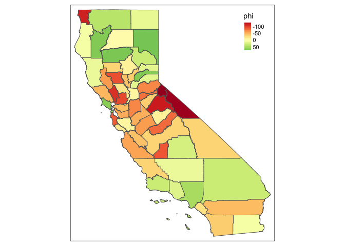
Id say that looks pretty dang autocorrelated! Let’s see:
morans <- function(shp, var){
  moran.test(pull(shp, var), nb2listw(poly2nb(shp),style="W", zero.policy=TRUE))
}
morans(CA_shp, "phi")

##
##  Moran I test under randomisation
##
## data:  pull(shp, var)
## weights: nb2listw(poly2nb(shp), style = "W", zero.policy = TRUE)
##
## Moran I statistic standard deviate = 4.4785, p-value = 3.758e-06
## alternative hypothesis: greater
## sample estimates:
## Moran I statistic       Expectation          Variance
##       0.359568078      -0.017543860       0.007090442
(If anyone knows a one-line command to do this directly in the SF package, let me know…. feels like there should be but I can’t tell?) Moran’s I is equal to 0.4 (p 1e-7), so I’d say that this worked.
I used a tiny value of τ here just for illustration. Let’s simulate with a bunch of different values of τ and see how the value of Moran’s I changes:
# Quick function to do this in one line

sim.f <- function(gamma, tau, CA_shp, adj, num, map = FALSE, summary = FALSE) {
  suppressWarnings({suppressMessages({
  simModel1 <- nimbleModel(code = simCode,
                        constants = list(n_counties = n_counties,
                                         adj = adj,
                                         n_adj = length(adj),
                                         num = num,
                                         tau = tau,
                                         gamma = gamma,
                                         mu = rep(0, n_counties)),
                        inits = inits)

  nodesToSim <- simModel1$getDependencies(c("phi"),self = T, downstream = T)
  simModel1$simulate(nodesToSim)
  simModel1$phi
  CA_shp$phi1 <- simModel1$phi
  })})

  if (map) {print(CA_shp %>% tm_shape() + tm_polygons(col =c("phi"), style = "cont"))}
  if (summary){return(morans(CA_shp, "phi1"))}
  return(morans(CA_shp, "phi1")$estimate[[1]])
}

sim.f(1, 0.99, CA_shp, adj, num, map = TRUE, summary = TRUE)

##
##  Moran I test under randomisation
##
## data:  pull(shp, var)
## weights: nb2listw(poly2nb(shp), style = "W", zero.policy = TRUE)
##
## Moran I statistic standard deviate = 6.3279, p-value = 1.243e-10
## alternative hypothesis: greater
## sample estimates:
## Moran I statistic       Expectation          Variance
##       0.512786604      -0.017543860       0.007023905
If you change gamma to something huge, the values change, but the Moran’s statistic doesn’t change dramatically.
What if you change the gamma parameter
sim.f(0.0001, 0.01, CA_shp, adj, num, map = TRUE, summary = TRUE)

##
##  Moran I test under randomisation
##
## data:  pull(shp, var)
## weights: nb2listw(poly2nb(shp), style = "W", zero.policy = TRUE)
##
## Moran I statistic standard deviate = -1.4702, p-value = 0.9292
## alternative hypothesis: greater
## sample estimates:
## Moran I statistic       Expectation          Variance
##      -0.140428189      -0.017543860       0.006986103
It doesn’t really change! This is really funky. Let’s step through a bunch of values of gamma and tau and see what we find. First, find the bounds on gamma:
carMinBound(
  C= CAR_calcC(adj, num),
  adj = adj,
  num = num,
  M = rep(1, 58))

## [1] -1.414268

carMaxBound(
  C= CAR_calcC(adj, num),
  adj = adj,
  num = num,
  M = rep(1, 58))

## [1] 1
Looks like rho/gamma need to be within -1.414 and 1. Let’s test:
gamma_vec <- seq(-1.414268, 1, length.out = 10)
tau_vec <- 10^(seq(-5, 2, length.out = 10))

df <- expand_grid(gamma_vec, tau_vec)
df$i <- 0


if (F) {
  for (i in 1:nrow(df)) {
    df[i, "i"]  <- sim.f(df[i, "gamma_vec"], df[i, "tau_vec"], CA_shp, adj, num)
  }
  save(df, file = "morans_df.Rdata")
} else {
  load("morans_df.Rdata")
}


ggplot(df) +
  geom_tile(aes(gamma_vec, tau_vec, fill = i), size = 10) +
  scale_y_continuous()
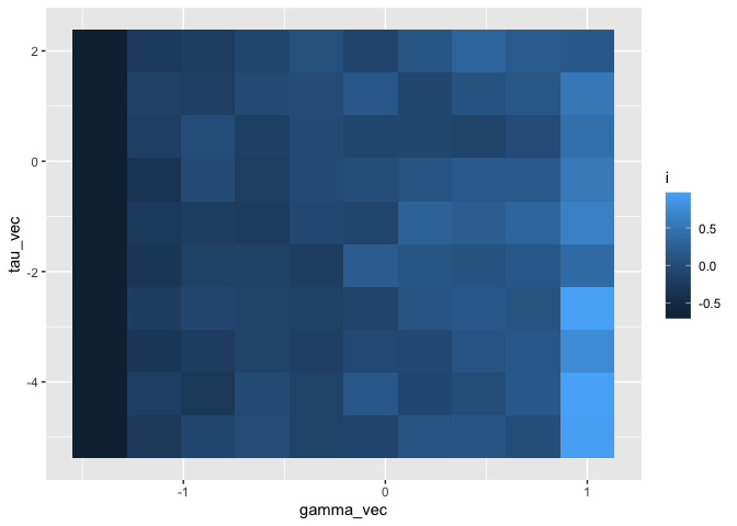
Okay, lighter values = higher Moran’s i, darker values = lower Moran’s i. There’s a pretty clear relationship with gamma: higher -> more autocorrelation, as expected. Remember, a higher value of gamma means that a higher proportion of the density is coming from the autoregressive ‘part’, and less is coming from the constant ‘part.’ But this relationship is obviously stronger when the precision is higher and less pronounced when it’s lower.
I don’t have a good answer for why that is! But it’s worth figuring out, I think.
Before I go to bed: a quick check of conditional independence between them:
independence_test(i ~ gamma_vec + tau_vec, data = df)

##
##  Asymptotic General Independence Test
##
## data:  i by gamma_vec, tau_vec
## maxT = 8.4529, p-value < 2.2e-16
## alternative hypothesis: two.sided
Nope! Not independent :+)